3. AstroLogics Tutorial, Boolean Network Analysis and Clustering : Invasion model

This tutorial demonstrates the AstroLogics framework for analyzing and comparing Boolean network model ensembles. AstroLogics is designed for benchmarking Boolean models through three major evaluation criteria: network evaluation, logical function evaluation, and dynamic evaluation.

3.1. Overview of AstroLogics Framework

AstroLogics addresses a critical gap in Boolean network modeling: while multiple methods exist for Boolean model synthesis (like Bonesis, BN-sketch), there hasn’t been a standardized way to evaluate and compare generated model ensembles. The framework focuses on:

• Dynamic properties: Examining state transition graphs and model behaviors through simulation

• Logical function evaluation: Analyzing and comparing logical rules that govern node behaviors

• Model clustering: Identifying groups of models with similar dynamics and logical features

3.2. Required Libraries

import pandas as pd
import os
import sys
import astrologics as ast
import seaborn as sns
import matplotlib.pyplot as plt

3.2.1. Dataset: Cancer Invasion model

We’ll use the Cancer Invasion model, which is more complex than the CNS differentiation model. This model contains 32 nodes with extensive connectivity and demonstrates key regulatory mechanisms involved in cancer cell invasion and metastasis processes. The model incorporates signaling pathways related to EMT (Epithelial-Mesenchymal Transition), cell adhesion, and extracellular matrix degradation.

This model has been used the demonstrate the capability of Bonesis and to introduce the concept of Boolean model ensemble, described here

3.3. Step 1: Load Model Ensemble

model_path = '../models/Invasion/'
model = ast.ensemble(model_path, project_name = 'Invasion')
model.create_simulation()

Simulation object created

The ensemble object is the core component of AstroLogics that handles:

• Loading multiple Boolean network models from a directory

• Managing simulation parameters and configurations

• Coordinating analysis across the model ensemble

3.4. Step 2: Simulate the model ensemble

In this part of the script we first simulate all the BN within the model ensemble. We utilize the MaBoSS engine as the main simulator.

Also, the use of MaBoSS also allows us to determine different intial states of the simulation. We then first look at the initial states which has been described in Chevalier & Noel et al., 2020.

# Read network structure and set initial conditions
test = pd.read_csv(model_path + 'Invasion_0.bnet', sep = ',', header = None)
test[1] = 0.5  # Set all nodes to 0.5 probability initially
test_dict = dict(zip(test[0], test[1]))

This creates an initial state where all nodes have equal probability (0.5) of being active. This represents a neutral starting condition that allows the system to evolve according to its inherent dynamics.

We then start the simulation using MaBoSS.

MaBoSS (Markovian Boolean Stochastic Simulator) is crucial for the AstroLogics approach because:

• It converts Boolean network dynamics into continuous-time Markov processes

• Provides probabilistic approximation of complex state transition graphs

• Enables analysis of both transient and steady-state behaviors

• Scales computationally better than exhaustive state space exploration

Simulation takes about 16 minutes (20-core 12th Gen Intel® Core™ i7-12700H × 20).

We therefore, added the simulated files in the tmp (the file is called Invasion_simulation_random.csv), which can be load directly into the model.simulation.simulation_df

# Configure simulation parameters
#model.simulation.update_parameters(max_time = 20,thread_count = 15, sample_count = 2000)
#model.simulation.run_simulation(initial_state=test_dict)
#model.simulation.simulation_df.to_csv('data/precomputed_Invasion_simulation_random.csv')

# Load the simulation results
model.simulation.simulation_df = pd.read_csv('../data/precomputed_Invasion_simulation_random.csv', index_col=0)

3.5. Step 3 : Calculate the trajectory and visualize the distance matrix using MDS

In this part of the script, we compare the two method of calculating the distance between models.

In this function calculate_distancematrix, users can select the two options of data used to calculate the distance.

• endpoint : The endpoint utilize the node activation probability at the endpoint of MaBoSS simulation. User could also defines the timepoint to define a specific timepoint they want to use to define the distance

• trajectory : This options utilize the whole MaBoSS simulation trajectory and the dtw method to calculate the distances between models.

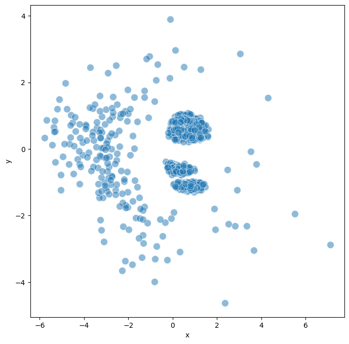
In this part, we show different results that could be obtained from two different method.

• Using endpoint we showed no clear separation of the model, which coresspond to the single attractors that all the model could reach.

• On the other hand, when using trajectory we can observe two major cluster of models based on the different signaling path that two groups of BNs took.

model.create_trajectory()

Trajectory object created

model.trajectory.calculate_distancematrix(mode = 'trajectory')
# Perform MDS (Multidimensional Scaling) for visualization
model.trajectory.calculate_MDS(random_state=12345)
model.trajectory.plot_MDS(s = 100, fig_size = (8,8))

Calculating distance matrix for whole trajectory...

Distance matrix calculated successfully.

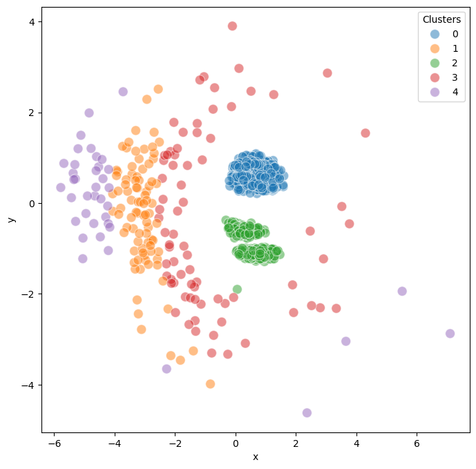
3.6. Step 4: Model Clustering

Clustering reveals distinct groups within the model ensemble. In this example, we found 2 major clusters corresponding to different attractor groups, representing distinct cellular fate decisions.

model.trajectory.calculate_kmean_cluster(n_cluster = 5, random_state = 12345)

Calculated k-means clustering with 5 clusters.

model.trajectory.plot_MDS(s = 100, fig_size = (8,8),plot_cluster = True, save_fig = True)

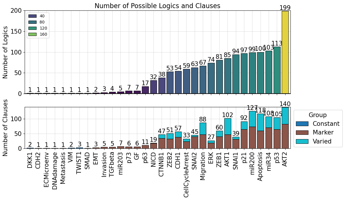
3.7. Step 5: Logic Function Analysis

This step implements the logical function evaluation component of AstroLogics:

• Converts Boolean equations to Disjunctive Normal Form (DNF)

• Creates feature matrices comparing logical rules across models

• Identifies constant, varied, and marker clauses

model.create_logic()
model.logic.model_logic
model.logic.create_flattend_logic_clause()

Loading models logics

Concatenate results into matrix

Logic object created
Flatten models logic clauses

Concatenate results into matrix

Flattend logic clause created

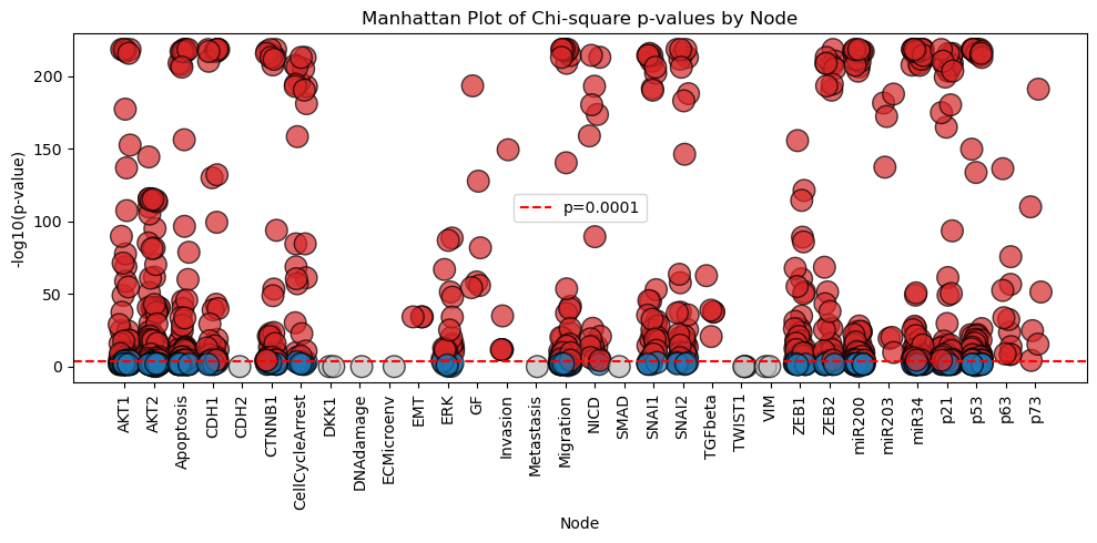
3.8. Step 6 : Calculate statistic of Logic features (clauses)

In this steps, we have already featurized the logical equations into model logics or clauses.

We can then integrate the clusters obtained from the trajectory analysis into the .logic and perform chi-square statistical test to categorize logic features (clauses) into 3 major groups

• Constatnt : core regulatory features that appears across BNs in the model ensemble

• Varied : Features that may differ between individual BNs but show no statistical significant

• Marker : Key discriminatory features that statistically distinguish between different model clusters.

We can define the p-value of the chi-square test using the function pval_threshold.

model.logic.map_model_clusters(model.trajectory.cluster_dict)
model.logic.calculate_logic_statistic(pval_threshold = 0.0001)

Model clusters mapped to logic clauses

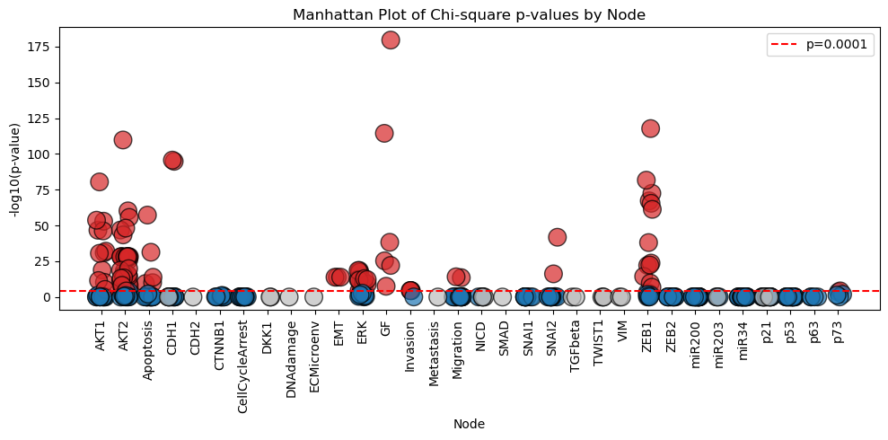
The results of the analysis can be visualized in the form of Manhattan Plot shown below.

model.logic.plot_manhattan()

Or the results can be summarized into the barplot shown here

model.logic.plot_logicstat_summary(save_fig = True)

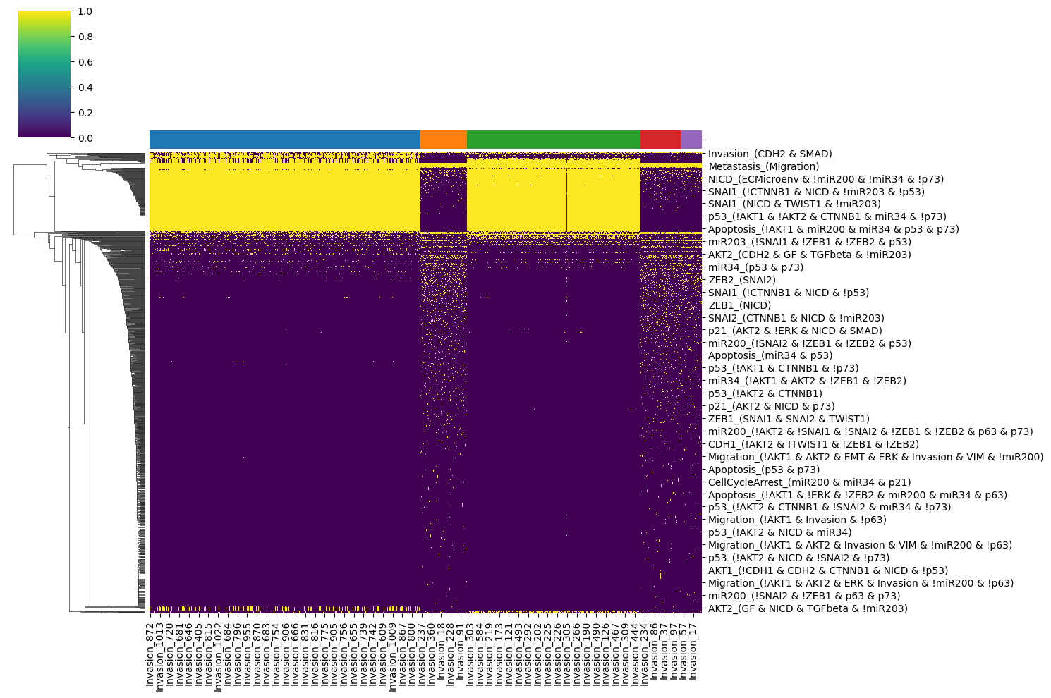
To have the overview of the process, we could plot the heatmap of the logical rules to see how different logical features in each model groups are.

logic_feature = model.logic.logic_clause_flattend
cluster_dict = model.trajectory.cluster_dict

# Map the cluster labels to the columns of the logic_feature
column_clusters = pd.Series(cluster_dict).reindex(logic_feature.columns, fill_value=-1)
column_clusters = column_clusters.sort_values()

# Create a color palette for the clusters
unique_clusters = column_clusters.unique()
palette = sns.color_palette("tab10", len(unique_clusters))
column_colors = column_clusters.map(dict(zip(unique_clusters, palette)))

# Create the clustermap
sns.clustermap(logic_feature[column_clusters.index], cmap='viridis', figsize=(15, 10),
               row_cluster=True, col_cluster=False, col_colors=column_colors)
plt.show()

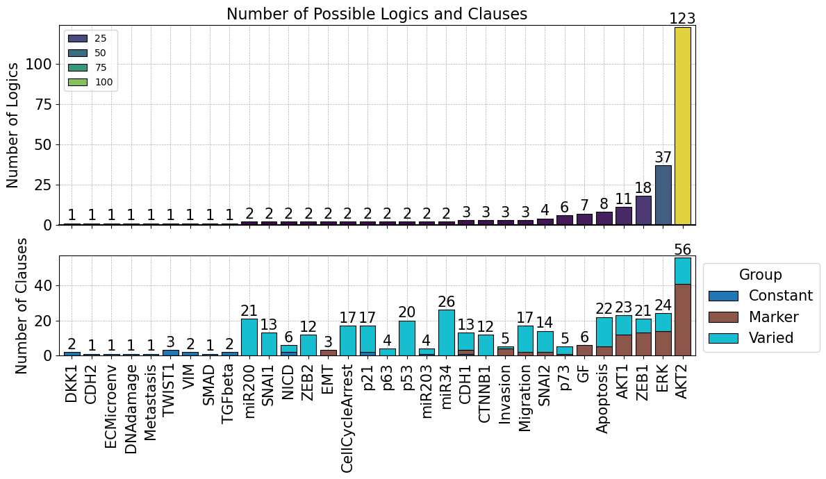
3.9. Step 7 : Subset models

In this part of the script, we found that the model can be clustered mainly into 2 main clusters; 0 and 2. We therefore, subset these models to perform the following logic analysis.

# Convert the cluster dictionary to a DataFrame
cluster_df = pd.DataFrame(list(cluster_dict.items()), columns=['Model_ID', 'Cluster'])
selected_model = cluster_df['Model_ID'][cluster_df['Cluster'].isin([0,2])]

# Subset the logic_feature DataFrame based on the selected models
model.logic.model_logic = model.logic.model_logic[selected_model]
model.logic.create_flattend_logic_clause()

Flatten models logic clauses

Concatenate results into matrix

Flattend logic clause created

# Subset the cluster dictionary based on the selected models
filtered_cluster_dict = {k: v for k, v in model.trajectory.cluster_dict.items() if k in set(selected_model)}

# Map the filtered cluster dictionary to the logic model
model.logic.map_model_clusters(filtered_cluster_dict)
model.logic.calculate_logic_statistic(pval_threshold = 0.0001)

Model clusters mapped to logic clauses

model.logic.plot_logicstat_summary(save_fig = True)

model.logic.plot_manhattan(show_label=False)

3.10. Step 7: Advanced Trajectory Analysis

These visualizations help identify:

• Most variable nodes: Components showing greatest differences between models

• Critical regulators: Nodes whose activity patterns distinguish model clusters

• Temporal patterns: How specific nodes behave over simulation time

In this first plot, we check what are the features that shows the highest variance in their dynamics accross simulation. We calculate the variance of node activation probabily of all BNs in the model ensemble across all timepoints and plotted using the heatmap.

model.trajectory.simulation_df = model.trajectory.simulation_df[model.trajectory.simulation_df.model_id.isin(selected_model)]

model.trajectory.plot_trajectory_variance()

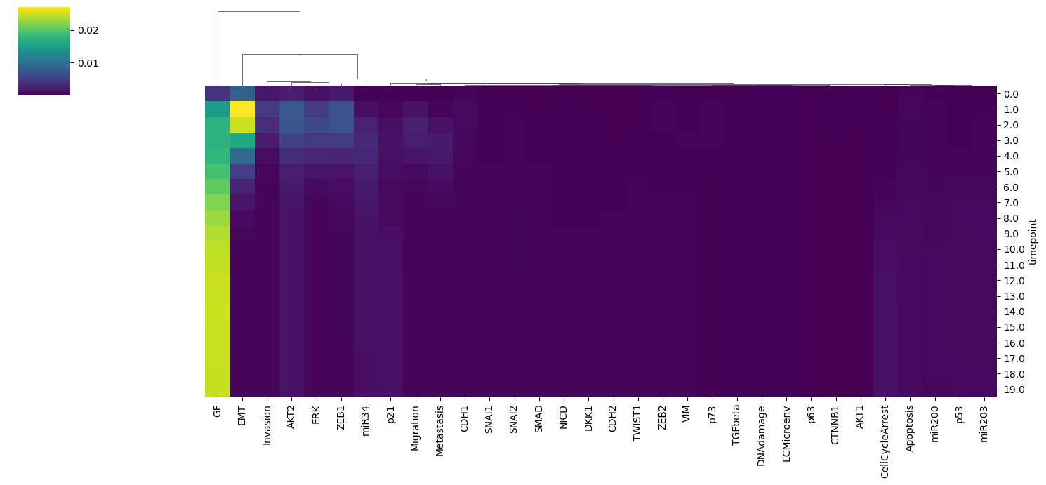
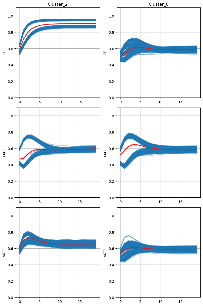
We identify the key node of interest (CDK46CycD) which shows the highest variance along the timepoints. Finally, we could visualize the dynamics of this node between two identified clusters using the lineplot.

From this, we found that the dynamics of this node differ during the early timepoint of the simulation, while finally converge to 0 at the later timepoint.

model.trajectory.plot_node_trajectory(node = ['GF', 'EMT', 'AKT2'],
                                      fig_width = 4, fig_height=4)

model.trajectory.plot_node_trajectory(node = ['GF'], fig_width = 4, fig_height = 4, save_fig = True)

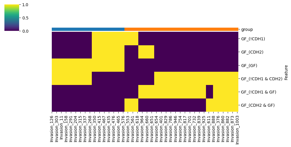
3.11. Step 8 : Logic Feature Heatmap

This analysis typically reveals that Myt1L is the key distinguishing node between clusters:

• Cluster 0: CDK46CycD is regulated by Bclaf1 & Myc

• Cluster 1: CDK46CycD is regulated by Bclaf1 | Myc

model.logic.plot_node_logic_heatmap(node = ['GF'],
                                     fig_size = (8, 8), save_fig = True)

<Figure size 800x800 with 0 Axes>